
Install Power BI Desktop
Power BI Desktop is a free Windows application from Microsoft. You do not need a Microsoft 365 subscription to build and view reports locally — a free Microsoft account is enough (and sign-in is only required to publish to the Power BI Service, not to build reports).
Option A — Microsoft Store (recommended)
- Press Win + S and type Microsoft Store, then open it.
- Search for Power BI Desktop.
- Click Get or Install. The Store version updates automatically in the background.
- Once installed, launch it from the Start menu.
Option B — Direct download from Microsoft
- Go to Microsoft's Power BI page and download the Power BI Desktop installer (search "download Power BI Desktop" to find the current download page).
- Run the
.exeinstaller and follow the setup wizard. - Launch Power BI Desktop from the Start menu or desktop shortcut.
Generate an API Key in Standard Time®
Every OData request to Standard Time® must include your API key. You generate it inside the application, copy it once, and paste it into every Power BI query. The key authenticates the request — think of it as a password for your data feed.
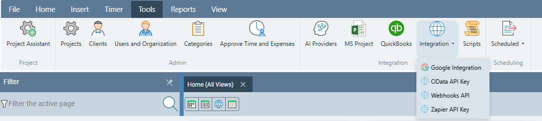
Step 1 — Open the OData API Key dialog
In Standard Time®, click the Tools tab in the ribbon. In the Integration panel, click the Integration dropdown and choose OData API Key.
Step 2 — Generate and copy your key
The OData API Key dialog lists your active keys. To create a new one:
- Type a descriptive Label (for example, Power BI) in the Label field, then click Change to save the label.
- Click Generate New Key. A new entry appears in the Active keys list showing the key's prefix (e.g.,
cN5YC4ZZ…) and its last-used date. - Copy the full key immediately — the complete key is displayed only at the moment of generation and cannot be retrieved again. Paste it into a secure text file or password manager right now.
- Click Close.
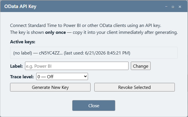
The dialog only displays a truncated preview of the key after generation. If you close the dialog without copying the full key, you must generate a new one. Multiple active keys are allowed — the old one keeps working until you click Revoke Selected.
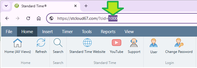
Find your Company ID (CID)
Every OData query also includes your company ID (CID), which appears in your Standard Time® cloud URL. CIDs are typically long alphanumeric strings — for example, if your Standard Time® web address is https://stcloud67.com/?cid=1000, then your CID is 1000, though real CIDs are usually much longer. Replace YOUR_CID_HERE in the queries below with your actual CID value.
1. Your API key (the long string you just generated)
2. Your CID (the number after
cid= in your Standard Time® URL, e.g., https://stcloud67.com/?cid=YOUR_CID_HERE)
How to Load Any OData Query
Each dashboard section below lists one or more M language query blocks. Use this same procedure for every query block you encounter.

Steps to paste a query into Power BI
- Open Power BI Desktop. Start with a new blank report.
- In the Home ribbon, click Get Data → Blank Query. The Power Query Editor window opens.
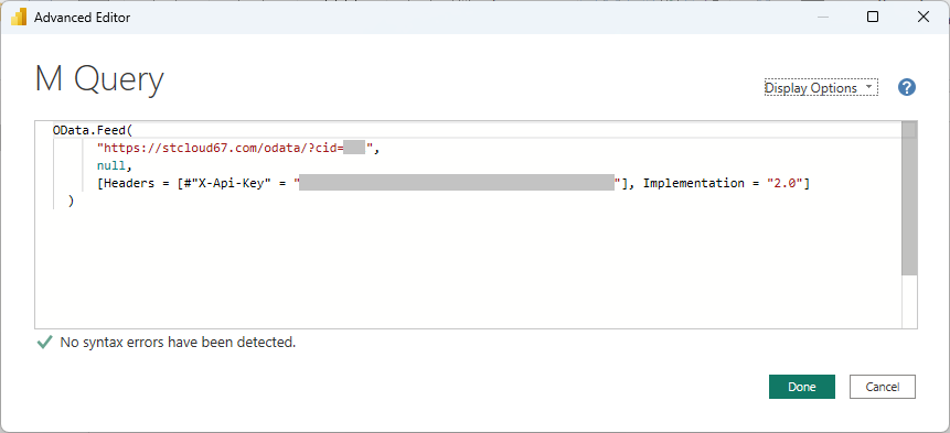
- In the Power Query Editor ribbon, click Home → Advanced Editor. A text editor opens with a simple placeholder query.
- Select all text in the editor (Ctrl+A), then paste the query block from this guide.
- Replace
YOUR_CID_HEREwith your actual CID — a long alphanumeric value found aftercid=in your Standard Time® cloud URL (e.g.,https://stcloud67.com/?cid=1000, though real CIDs are typically longer). - Replace
YOUR_APIKEYwith your full API key string. - Click Done. Power BI connects to Standard Time® and previews the data.
- In the left panel (Queries pane), right-click the query → Rename and type the name shown above each query block (e.g., TimeLogs).
- Repeat from step 2 for each additional query in the dashboard section.
- When all queries for a dashboard are loaded, click Close & Apply in the Power Query ribbon to import the data into Power BI.
DaysBack variable) recalculate automatically on every refresh.
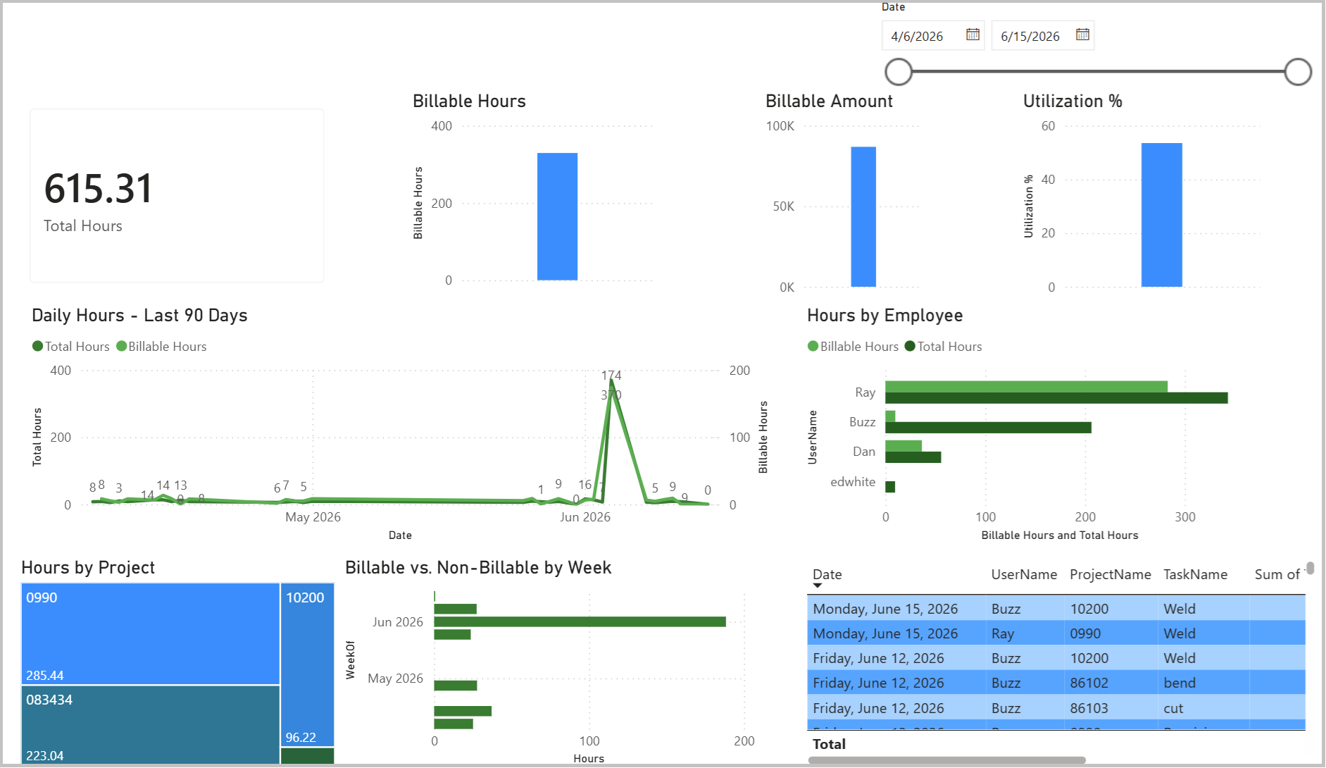
Dashboard 1 — Shop Floor Time & Utilization Command Center
Every hour logged on the shop floor — who worked, on which job, in which category, and whether that time is billable. At a glance managers see total hours, billable vs. non-billable split, daily output trend, which employees are most utilized, and which projects are consuming the most time. Designed to be left on a monitor in the production office and refreshed daily.
Step 1 — Load the data
Load all three queries using the procedure above. Name each query exactly as shown.
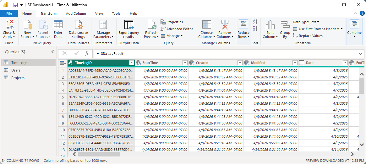
Query: TimeLogs
let
    DaysBack = 90,

    Cutoff = DateTimeZone.ToText(
        DateTimeZone.LocalNow() - #duration(DaysBack, 0, 0, 0),
        "yyyy-MM-ddTHH:mm:sszzz"
    ),

    Source = OData.Feed(
        "https://stcloud67.com/odata/TimeLogs?cid=YOUR_CID_HERE&$filter=Created gt " & Cutoff,
        null,
        [Headers = [#"X-Api-Key" = "YOUR_APIKEY"]]
    )
in
    Source
Query: Users
let
    Source = OData.Feed(
        "https://stcloud67.com/odata/Users?cid=YOUR_CID_HERE",
        null,
        [Headers = [#"X-Api-Key" = "YOUR_APIKEY"]]
    )
in
    Source
Query: Projects
let
    DaysBack = 9999,

    Cutoff = DateTimeZone.ToText(
        DateTimeZone.LocalNow() - #duration(DaysBack, 0, 0, 0),
        "yyyy-MM-ddTHH:mm:sszzz"
    ),

    Source = OData.Feed(
        "https://stcloud67.com/odata/Projects?cid=YOUR_CID_HERE&$filter=Created gt " & Cutoff,
        null,
        [Headers = [#"X-Api-Key" = "YOUR_APIKEY"]]
    )
in
    Source
Step 2 — Create calculated columns and measures
In Power BI Desktop, click the TimeLogs table in the Data/Fields pane on the right. Use Table Tools → New Column for calculated columns and Home → New Measure for measures.
Create the WeekOf calculated column first (groups logs by calendar week):
New Column on TimeLogs — WeekOf
WeekOf = DATE(YEAR(TimeLogs[Date]), MONTH(TimeLogs[Date]),
    DAY(TimeLogs[Date]) - WEEKDAY(TimeLogs[Date], 2) + 1)
Then add these measures:
New Measure — Total Hours
Total Hours = SUM(TimeLogs[TimeLogDurationHours])
New Measure — Billable Hours
Billable Hours = CALCULATE(SUM(TimeLogs[TimeLogDurationHours]), TimeLogs[Billable] = TRUE())
New Measure — Non-Billable Hours
Non-Billable Hours = [Total Hours] - [Billable Hours]
New Measure — Billable Amount
Billable Amount = SUM(TimeLogs[TimeLogCostClient])
New Measure — Utilization %
Utilization % = DIVIDE([Billable Hours], [Total Hours], 0) * 100
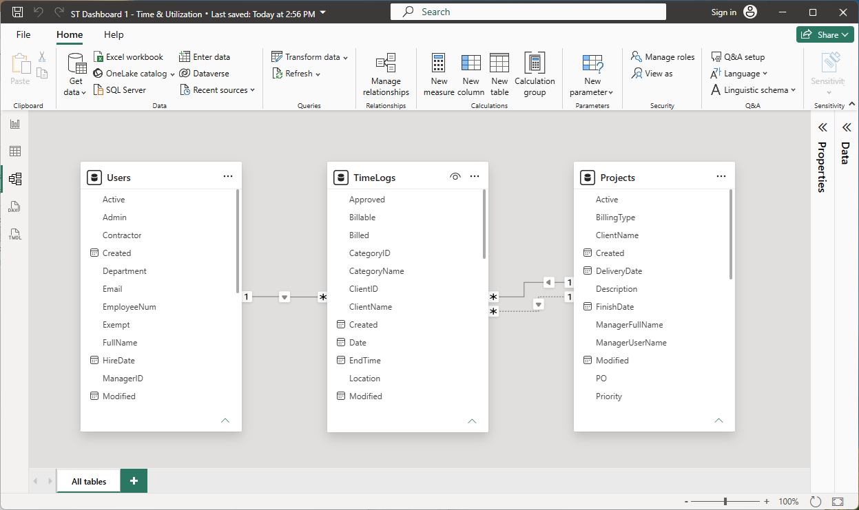
Step 3 — Set up table relationships
Click the Model icon in the left rail (the branching-diagram icon, third from the top). You should see three boxes on the canvas for TimeLogs, Users, and Projects.
- In the TimeLogs box, click and drag the UserID column onto the UserID column in the Users box. An Edit Relationship dialog opens — verify Many-to-One (*:1), Single direction, Active. Click OK.
- In the TimeLogs box, drag ProjectID onto ProjectID in the Projects box. Verify Many-to-One, Single, Active. Click OK.
- Both connections show as solid lines with a * on the TimeLogs side and a 1 on the Users/Projects side.
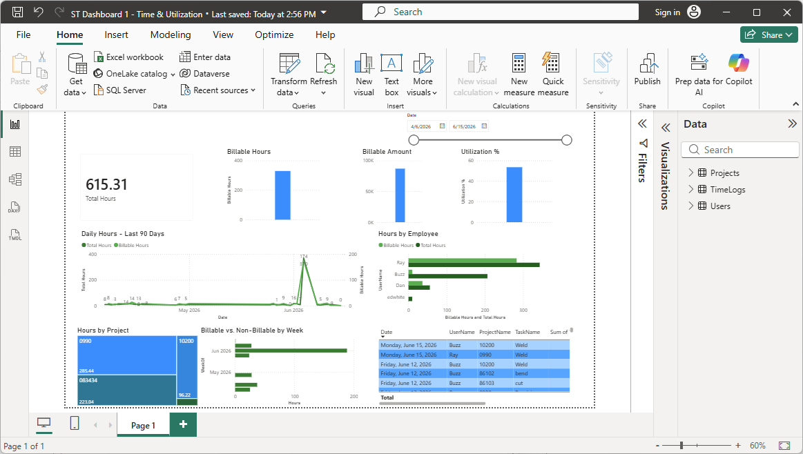
Step 4 — Build the report page
Click the Report icon (bar chart, top of the left rail) to return to Report view. Build the following seven visuals. For each one: click an empty area of the canvas, click the visual type in the Visualizations pane, then drag fields from the Data pane into the correct wells.
| Visual | Type | Fields | Format notes |
|---|---|---|---|
| KPI Cards (×4) | Card | Total Hours · Billable Hours · Billable Amount · Utilization % | Callout value font 28pt bold. For Billable Amount: set format to Currency in Data pane. For Utilization %: 1 decimal place. |
| Daily Hours Trend | Line chart | X-axis: TimeLogs[Date] (flat, not hierarchy)Y-axis: Total Hours Secondary Y: Billable Hours |
Line colors: Total Hours = #2e7d32, Billable Hours = #4caf50. Stroke width 2.5. Title: "Daily Hours — Last 90 Days". |
| Hours by Employee | Clustered bar chart | Y-axis: Users[FullName]X-axis: Total Hours, Billable Hours |
Colors: Total Hours = #1b5e20, Billable Hours = #4caf50. Sort by Total Hours desc (⋯ → Sort axis → Sort descending). Title: "Hours by Employee". |
| Hours by Project | Treemap | Category: TimeLogs[ProjectName]Values: Total Hours |
Data colors: diverging scale, max = #1b5e20. Data labels on. Title: "Hours by Project". |
| Billable vs. Non-Billable by Week | Stacked bar chart | Y-axis: TimeLogs[WeekOf]X-axis: Billable Hours, Non-Billable Hours |
Colors: Billable = #2e7d32, Non-Billable = #e0e0e0. Title: "Billable vs. Non-Billable by Week". |
| Date Range Slicer | Slicer | Field: TimeLogs[Date] |
Format tab → Slicer settings → Style: Between. Place in a corner near the KPI cards. |
| Detail Table | Table | TimeLogs[Date], Users[FullName], TimeLogs[ProjectName], TimeLogs[TaskName], TimeLogs[CategoryName], TimeLogs[TimeLogDurationHours], TimeLogs[Billable], TimeLogs[TimeLogCostClient] |
Sort Date desc. Header bg #2e7d32, font white, 11pt bold. Alternate row color #f1f8e9. Span full canvas width at bottom. |
Step 5 — Finish and save
- Add a Text Box at the top: "Shop Floor Time & Utilization" — 20pt bold, color
#2e7d32. - Set page background: View → Page background → white (
#FFFFFF). - File → Save as
ST Dashboard 1 - Time & Utilization.pbix
Dashboard 2 — Project Budget vs. Actuals
For every active project: how many hours were estimated, how many have been used, how much is remaining, and whether the project is tracking under or over its quoted cost. A scatter plot reveals which projects are burning hours faster than they're progressing. Built for project managers who need to answer "are we on budget?" before a client call.
Step 1 — Load the data
Query: Projects
let
    DaysBack = 9999,

    Cutoff = DateTimeZone.ToText(
        DateTimeZone.LocalNow() - #duration(DaysBack, 0, 0, 0),
        "yyyy-MM-ddTHH:mm:sszzz"
    ),

    Source = OData.Feed(
        "https://stcloud67.com/odata/Projects?cid=YOUR_CID_HERE&$filter=Created gt " & Cutoff,
        null,
        [Headers = [#"X-Api-Key" = "YOUR_APIKEY"]]
    )
in
    Source
Query: ProjectTasks
let
    DaysBack = 9999,

    Cutoff = DateTimeZone.ToText(
        DateTimeZone.LocalNow() - #duration(DaysBack, 0, 0, 0),
        "yyyy-MM-ddTHH:mm:sszzz"
    ),

    Source = OData.Feed(
        "https://stcloud67.com/odata/ProjectTasks?cid=YOUR_CID_HERE&$filter=Created gt " & Cutoff,
        null,
        [Headers = [#"X-Api-Key" = "YOUR_APIKEY"]]
    )
in
    Source
Query: Clients
let
    Source = OData.Feed(
        "https://stcloud67.com/odata/Clients?cid=YOUR_CID_HERE",
        null,
        [Headers = [#"X-Api-Key" = "YOUR_APIKEY"]]
    )
in
    Source
Step 2 — Create measures and columns
Select the Projects table in the Data pane, then create the following measures and column.
New Measure — Avg % Complete
Avg % Complete = AVERAGEX(ProjectTasks, ProjectTasks[PercentComplete])
New Measure — Total Quoted Cost
Total Quoted Cost = SUM(Projects[ProjectQuotedCost])
New Measure — Total Actual Billable
Total Actual Billable = SUM(ProjectTasks[TaskCostClientActual])
New Measure — Budget Variance
Budget Variance = [Total Quoted Cost] - [Total Actual Billable]
New Measure — Budget Used %
Budget Used % = DIVIDE([Total Actual Billable], [Total Quoted Cost], 0) * 100
New Measure — Total Actual Hours
Total Actual Hours = SUM(ProjectTasks[ActualHours])
New Measure — Total Estimated Hours
Total Estimated Hours = SUM(ProjectTasks[TaskDurationHours])
New Measure — Total Remaining Hours
Total Remaining Hours = SUM(ProjectTasks[RemainingHours])
Add this calculated column to the Projects table (Table Tools → New Column):
New Column on Projects — Health Status
Health Status =
VAR pct = DIVIDE(
    CALCULATE(SUM(ProjectTasks[TaskCostClientActual]),
              ProjectTasks[ProjectID] = Projects[ProjectID]),
    Projects[ProjectQuotedCost], 0) * 100
RETURN
    IF(pct > 100, "Over Budget",
    IF(pct > 80,  "At Risk",
                  "On Track"))
Step 3 — Set up relationships
In Model view, create these connections (all Many-to-One, Single direction, Active):
- Drag ProjectTasks[ProjectID] → Projects[ProjectID]
- Drag Projects[ClientID] → Clients[ClientID]
Step 4 — Build the report page
| Visual | Type | Fields | Format notes |
|---|---|---|---|
| KPI Cards (×4) | Card | Total Estimated Hours · Total Actual Hours · Total Remaining Hours · Budget Used % | Budget Used %: 1 decimal, no % symbol needed (the name says it). |
| Quoted Cost vs. Actual Billable | Clustered bar chart | Y-axis: Projects[ProjectName]X-axis: Total Quoted Cost ( #1b5e20), Total Actual Billable (#4caf50) |
Sort by Quoted Cost desc. Enable data labels. Title: "Quoted Cost vs. Actual Billable Amount". |
| Hour Burn: Used vs. Remaining | Stacked bar chart | Y-axis: Projects[ProjectName]Values: Total Actual Hours ( #2e7d32), Total Remaining Hours (#a5d6a7) |
Title: "Hour Burn — Used vs. Remaining". |
| Budget vs. Progress Scatter | Scatter chart | X-axis: Budget Used % Y-axis: Avg % Complete Size: Total Estimated Hours Details: Projects[ProjectName] |
Add constant lines at X=50 and Y=50 (Analytics pane) to create quadrants. Title: "Budget Consumed vs. Progress". |
| Project Health Matrix | Matrix | Rows: Projects[ProjectName]Values: Health Status, Total Estimated Hours, Total Actual Hours, Budget Used %, Projects[FinishDate] |
Conditional formatting on Health Status: "Over Budget" → bg #ffcdd2, "At Risk" → #fff9c4, "On Track" → #c8e6c9. |
| Task % Complete | Bar chart | Y-axis: ProjectTasks[TaskName]X-axis: ProjectTasks[PercentComplete] |
Title: "Task % Complete (select a project in the health matrix to filter)". |
| Slicers (×2) | Slicer | Projects[Status] and Clients[CompanyName] |
Dropdown or list style. Place in a sidebar or top strip. |
Step 5 — Finish and save
Page background: very light green #f1f8e9. Title text box: "Project Budget vs. Actuals" — 20pt bold #1b5e20. Save as ST Dashboard 2 - Project Budget.pbix.
Dashboard 3 — Full Job Cost Command Center (Labor + Materials)
The complete picture of what a job actually costs: hours × rate for labor, plus every material and expense charged against the project. Standard Time®'s Expenses table captures every inventory scan and manual expense entry, so this dashboard shows true job cost (labor + materials) in one view. Managers can answer "how much did job #47 really cost us?" including parts consumed and mileage.
Step 1 — Load the data
Query: TimeLogs
let
    DaysBack = 365,

    Cutoff = DateTimeZone.ToText(
        DateTimeZone.LocalNow() - #duration(DaysBack, 0, 0, 0),
        "yyyy-MM-ddTHH:mm:sszzz"
    ),

    Source = OData.Feed(
        "https://stcloud67.com/odata/TimeLogs?cid=YOUR_CID_HERE&$filter=Created gt " & Cutoff,
        null,
        [Headers = [#"X-Api-Key" = "YOUR_APIKEY"]]
    )
in
    Source
Query: Expenses
let
    DaysBack = 365,

    Cutoff = DateTimeZone.ToText(
        DateTimeZone.LocalNow() - #duration(DaysBack, 0, 0, 0),
        "yyyy-MM-ddTHH:mm:sszzz"
    ),

    Source = OData.Feed(
        "https://stcloud67.com/odata/Expenses?cid=YOUR_CID_HERE&$filter=Created gt " & Cutoff,
        null,
        [Headers = [#"X-Api-Key" = "YOUR_APIKEY"]]
    )
in
    Source
Query: Projects
let
    DaysBack = 9999,

    Cutoff = DateTimeZone.ToText(
        DateTimeZone.LocalNow() - #duration(DaysBack, 0, 0, 0),
        "yyyy-MM-ddTHH:mm:sszzz"
    ),

    Source = OData.Feed(
        "https://stcloud67.com/odata/Projects?cid=YOUR_CID_HERE&$filter=Created gt " & Cutoff,
        null,
        [Headers = [#"X-Api-Key" = "YOUR_APIKEY"]]
    )
in
    Source
Query: Clients
let
    Source = OData.Feed(
        "https://stcloud67.com/odata/Clients?cid=YOUR_CID_HERE",
        null,
        [Headers = [#"X-Api-Key" = "YOUR_APIKEY"]]
    )
in
    Source
Step 2 — Build the unified CostLines table
This is the key step that makes Dashboard 3 unique: merging TimeLogs and Expenses into a single CostLines table so every visual can show combined labor + material cost in one view.
- In Power BI Desktop, click Home → Transform data to open Power Query Editor.
- In the ribbon, click Home → Append Queries → Append Queries as New.
- Choose Two tables: Primary = TimeLogs, Secondary = Expenses. Click OK.
- In the Queries pane on the left, right-click the new query and rename it CostLines.
- With CostLines selected, click Add Column → Custom Column. Name it CostType and enter this formula:
if [TimeLogDurationHours] = null then "Material" else "Labor"
- Add a second custom column. Name it CostAmount:
if [CostType] = "Labor" then [TimeLogCostClient] else [ExpenseAmount]
- Click Close & Apply.
Step 3 — Create measures
Select the CostLines table:
New Measure — Total Labor Cost
Total Labor Cost =
CALCULATE(SUM(CostLines[CostAmount]), CostLines[CostType] = "Labor")
New Measure — Total Material Cost
Total Material Cost =
CALCULATE(SUM(CostLines[CostAmount]), CostLines[CostType] = "Material")
New Measure — Total Job Cost
Total Job Cost = [Total Labor Cost] + [Total Material Cost]
New Measure — Labor %
Labor % = DIVIDE([Total Labor Cost], [Total Job Cost], 0) * 100
New Measure — Material %
Material % = DIVIDE([Total Material Cost], [Total Job Cost], 0) * 100
Select the Expenses table:
New Measure — Unbilled Expenses
Unbilled Expenses =
CALCULATE(SUM(Expenses[ExpenseAmount]),
    Expenses[Billable] = TRUE(),
    Expenses[Billed] = FALSE())
New Measure — Pending Reimbursements
Pending Reimbursements =
CALCULATE(SUM(Expenses[ExpenseAmount]),
    Expenses[Reimbursable] = TRUE(),
    Expenses[Reimbursed] = FALSE())
Add a MonthYear calculated column to CostLines for the monthly trend chart (Table Tools → New Column):
New Column on CostLines — MonthYear
MonthYear = FORMAT(
    IF(NOT(ISBLANK(CostLines[Date])), CostLines[Date], CostLines[ExpenseDate]),
    "YYYY-MM"
)
Step 4 — Set up relationships
In Model view (all Many-to-One, Single, Active):
- Drag TimeLogs[ProjectID] → Projects[ProjectID]
- Drag Expenses[ProjectID] → Projects[ProjectID]
- Drag Expenses[ClientID] → Clients[ClientID]
- Drag Projects[ClientID] → Clients[ClientID]
Step 5 — Build the report page
| Visual | Type | Fields | Format notes |
|---|---|---|---|
| KPI Cards (×5) | Card | Total Labor Cost · Total Material Cost · Total Job Cost · Unbilled Expenses · Pending Reimbursements | Currency format on all five. For Unbilled Expenses: conditional formatting → if value > 0, font color = #c62828 (red). |
| Job Cost by Project | Stacked bar chart | Y-axis: CostLines[ProjectName]X-axis: Total Labor Cost ( #2e7d32), Total Material Cost (#ff8f00 amber) |
Sort by Total Job Cost desc. Title: "Job Cost by Project — Labor vs. Materials". |
| Labor vs. Material Split | Clustered column chart | X-axis: CostLines[CostType]Y-axis: Total Job Cost |
Colors: Labor = #2e7d32, Material = #ff8f00. Title: "Labor vs. Material Split". |
| Monthly Job Cost Trend | Area chart | X-axis: CostLines[MonthYear]Y-axis: Total Labor Cost ( #2e7d32), Total Material Cost (#ff8f00) |
Title: "Monthly Job Cost Trend". |
| Client Billing Summary | Matrix | Rows: Clients[CompanyName] → Projects[ProjectName]Values: Total Labor Cost, Total Material Cost, Total Job Cost |
Enable subtotals per client. Conditional formatting on Total Job Cost: data bars, max color #2e7d32. |
| Top Materials Charged | Table | Filter to CostLines[CostType] = "Material"Columns: Expenses[InventoryName], Expenses[CategoryName], SUM(ExpenseQty), SUM(ExpenseAmount) |
Sort by ExpenseAmount desc. Title: "Top Materials Charged to Jobs". |
| Slicers (×4) | Slicer | Clients[CompanyName] · Projects[Status] · CostLines[CostType] · Date range on CostLines[Date] |
Date range slicer: Format → Slicer settings → Style: Between. |
Step 6 — Finish and save
Page background: near-white warm #FFFFF8. Title text box: "Full Job Cost — Labor + Materials" — 20pt bold #1b5e20. Use amber (#ff8f00) consistently for all material visuals to distinguish from labor green. Save as ST Dashboard 3 - Job Cost.pbix.
Dashboard 4 — Inventory Health & Consumption Radar
A live view of shop floor inventory: what's in stock, what's falling below the reorder threshold, how much each item costs, and which materials are being consumed fastest (tracked via Expenses records created by barcode scans). Items in red need ordering before production stalls.
Step 1 — Load the data
Query: Inventory
let
    Source = OData.Feed(
        "https://stcloud67.com/odata/Inventory?cid=YOUR_CID_HERE",
        null,
        [Headers = [#"X-Api-Key" = "YOUR_APIKEY"]]
    )
in
    Source
Query: MaterialScans
Fetches the last 90 days of Expense records where InventoryName is not blank — these are material consumption events created by inventory barcode scans.
let
    DaysBack = 90,

    Cutoff = DateTimeZone.ToText(
        DateTimeZone.LocalNow() - #duration(DaysBack, 0, 0, 0),
        "yyyy-MM-ddTHH:mm:sszzz"
    ),

    Source = OData.Feed(
        "https://stcloud67.com/odata/Expenses?cid=YOUR_CID_HERE&$filter=Created gt " & Cutoff,
        null,
        [Headers = [#"X-Api-Key" = "YOUR_APIKEY"]]
    ),

    MaterialScans = Table.SelectRows(Source, each [InventoryName] <> null and [InventoryName] <> "")
in
    MaterialScans
Query: Projects
let
    DaysBack = 9999,

    Cutoff = DateTimeZone.ToText(
        DateTimeZone.LocalNow() - #duration(DaysBack, 0, 0, 0),
        "yyyy-MM-ddTHH:mm:sszzz"
    ),

    Source = OData.Feed(
        "https://stcloud67.com/odata/Projects?cid=YOUR_CID_HERE&$filter=Created gt " & Cutoff,
        null,
        [Headers = [#"X-Api-Key" = "YOUR_APIKEY"]]
    )
in
    Source
Step 2 — Create calculated columns
Select the Inventory table (Table Tools → New Column for each):
New Column — Stock Status
Stock Status =
IF(Inventory[QtyInStock] <= 0, "Out of Stock",
IF(Inventory[QtyInStock] <= Inventory[QtyWhenToReorder], "Reorder Now",
IF(Inventory[QtyInStock] <= Inventory[QtyWhenToReorder] * 1.25, "Low",
   "OK")))
New Column — Inventory Value
Inventory Value = Inventory[QtyInStock] * Inventory[CostUnit]
New Column — Margin Per Unit
Margin Per Unit = Inventory[CostClient] - Inventory[CostUnit]
New Column — Stock Gap
Stock Gap =
IF(Inventory[QtyInStock] < Inventory[QtyWhenToReorder],
   Inventory[QtyWhenToReorder] - Inventory[QtyInStock],
   0)
Step 3 — Create measures
Select the Inventory table:
New Measure — Total Inventory Value
Total Inventory Value = SUMX(Inventory, Inventory[QtyInStock] * Inventory[CostUnit])
New Measure — Items Below Reorder
Items Below Reorder =
CALCULATE(
    COUNTROWS(Inventory),
    Inventory[QtyInStock] <= Inventory[QtyWhenToReorder],
    Inventory[Active] = TRUE()
)
New Measure — Items Out of Stock
Items Out of Stock =
CALCULATE(
    COUNTROWS(Inventory),
    Inventory[QtyInStock] <= 0,
    Inventory[Active] = TRUE()
)
Select the MaterialScans table:
New Measure — Total Units Consumed (90 days)
Total Units Consumed = SUM(MaterialScans[ExpenseQty])
New Measure — Total Material Cost (90 days)
Total Material Cost 90d = SUM(MaterialScans[ExpenseAmount])
Step 4 — Set up relationships
In Model view (all Many-to-One, Single, Active):
- Drag MaterialScans[InventoryName] → Inventory[Name]
- Drag MaterialScans[ProjectID] → Projects[ProjectID]
InventoryCode → Inventory[Code] instead.Step 5 — Build the report page
| Visual | Type | Fields | Format notes |
|---|---|---|---|
| KPI Cards (×5) | Card | Total Inventory Value · Items Below Reorder · Items Out of Stock · Total Units Consumed · Total Material Cost 90d | Currency on Value and Cost 90d. Conditional formatting on Items Below Reorder and Items Out of Stock: if value > 0, font color = #c62828 (red). |
| Stock Level vs. Reorder Point | Clustered bar chart | Y-axis: Inventory[Name]X-axis: SUM(QtyInStock) ( #2e7d32), SUM(QtyWhenToReorder) (#e53935 red) |
Filter to Active = TRUE. Sort by QtyInStock ascending (most critical at top). Title: "Stock Level vs. Reorder Point". |
| Items Requiring Action | Table | Inventory[Name], SKU, Vendor, QtyInStock, QtyWhenToReorder, Stock Gap, LeadTimeDays |
Filter: Stock Status is "Out of Stock" or "Reorder Now". Sort by Stock Gap desc. Conditional bg on Name: Out of Stock → #ffcdd2, Reorder Now → #fff9c4. |
| Top Consumed Items (90d) | Bar chart | Y-axis: MaterialScans[InventoryName]X-axis: Total Units Consumed |
Sort desc, show top 15. Data color: #ff8f00 amber. Title: "Top Consumed Items — Last 90 Days". |
| Cost vs. Stock Bubble Chart | Scatter chart | X-axis: SUM(CostUnit) Y-axis: SUM(QtyInStock) Size: SUM(Inventory Value) Details: Inventory[Name] |
Add reference lines at X = average unit cost and Y = 0 (Analytics pane). Items in lower-right (high cost, low stock) need immediate action. Title: "Unit Cost vs. Stock Level". |
| Material Cost by Job | Bar chart | Y-axis: MaterialScans[ProjectName]X-axis: Total Material Cost 90d |
Sort desc. Title: "Material Cost by Job (last 90 days)". |
| Inventory Health Donut | Donut chart | Legend: Inventory[Stock Status]Values: COUNTROWS(Inventory) |
Colors: Out of Stock → #c62828, Reorder Now → #e65100, Low → #fbc02d, OK → #2e7d32. Title: "Inventory Health by Status". |
| Slicers (×4) | Slicer | Inventory[Vendor] · Inventory[BuyOrBuild] · Inventory[Stock Status] · Inventory[Active] |
Set Active slicer default to TRUE so inactive items are hidden by default. |
Step 6 — Finish and save
Page background: warm light yellow #FFFDE7. Title text box: "Inventory Health & Consumption Radar" — 20pt bold. Use red/amber/green consistently: green = healthy, amber = watch, red = act now. Save as ST Dashboard 4 - Inventory Radar.pbix.
OData Column Quick Reference
Key columns available from each Standard Time® OData endpoint. Use these to add additional fields to visuals or build custom measures.
| Entity | Key Columns for Dashboards |
|---|---|
| TimeLogs | Date, TimeLogDurationHours, TimeLogCostClient, TimeLogCostSalary, TimeLogClientRate, Billable, Billed, Approved, UserName, TimeLogUserFullName, ProjectName, TaskName, CategoryName |
| Projects | ProjectName, Status, Active, StartDate, FinishDate, ProjectQuotedCost, ProjectClientRate, ProjectSalaryRate, ClientName, ManagerFullName, ProjectFolder |
| ProjectTasks | TaskName, PercentComplete, Completed, Billable, TaskDurationHours, ActualHours, RemainingHours, TaskCostClientActual, TaskCostClientRemain, TaskQuotedCost, StartDate, FinishDate, TaskDueDate |
| Expenses | ExpenseDate, ExpenseAmount, ExpenseQty, Price, Billable, Billed, Reimbursable, Approved, InventoryName, InventoryCode, ProjectName, CategoryName, Description |
| Inventory | Name, Code, QtyInStock, QtyWhenToReorder, QtyToReorder, CostUnit, CostClient, BuyOrBuild, Vendor, LeadTimeDays, SKU, Active, InventoryFolder |
| Users | UserName, FullName, Department, Workgroup, UserClientRate, UserSalaryRate, Active, Contractor, UserRoleName |
| Clients | CompanyName, Status, Active, MainContact, MainCity, MainState, ClientTaxRate, ClientFolder |
| Invoices | InvoiceNum, DateSent, InvoiceDueDate, DatePaid, InvoiceAmount, BalanceDue, PaidInFull, ClientName, ProjectName |
| BillingRates | RateType, BillingRateClientRate, BillingRateSalaryRate, StartDate, EndDate, UserName, ProjectName, CategoryName |
| Categories | Name, CategoryClientRate, CategorySalaryRate, Active, CategoryFolder |
Tips & Troubleshooting
| Problem | Solution |
|---|---|
| Refresh fails with 401 Unauthorized | Your API key is wrong or was revoked. In Standard Time®: View → OData API Key → Generate a new key, update every YOUR_APIKEY placeholder in Power Query (Home → Transform Data → Advanced Editor for each query). |
| No data returned / empty visuals | Increase DaysBack in the query (e.g., change 90 to 9999 to load all history). Click Home → Refresh in Power BI Desktop after any query change. |
| Decimal/hours columns show as text | In Power Query Editor (Home → Transform Data), select the column (e.g., TimeLogDurationHours) and set Data Type → Decimal Number in the Transform ribbon. |
| Relationship shows many-to-many warning | Verify your Projects or Users query isn't returning duplicate rows. Add &$top=5 temporarily to inspect a small sample. Look for any duplicate ProjectID or UserID values in the "one" side table. |
| Date slicer dates in wrong order | Right-click the date column in the Data pane → Sort by Column → choose the same date column. |
| KPI Cards show "(Blank)" | The measure returns no rows for the current filter context. Check that your DaysBack window covers the date range selected in the slicer. If using a date hierarchy, switch the slicer field from hierarchy to the flat date field. |
| WeekOf column not visible in Fields pane | Calculated columns appear after all source columns alphabetically — scroll to the bottom of the TimeLogs field list. If still missing, confirm you saved the column formula in Step 2 of Dashboard 1 (it should show up under TimeLogs, not Measures). |
| Users[FullName] shows "(Blank)" in detail table | The TimeLogs→Users relationship is missing or the UserID values do not match. Open Model view and verify the solid line between TimeLogs and Users exists with a star (*) on the TimeLogs side. |
| Inventory bubble chart — items overlap | Use Format → Bubbles → Max bubble size to reduce bubble size. You can also add a slicer on Inventory[Vendor] or Stock Status to focus on a subset. |
.pbix file to the Power BI Service (free Microsoft account required), configure a data gateway if needed, and set a scheduled refresh in the Power BI Service workspace settings. The OData feed URL and API key are stored in the published dataset's credentials.
OData & Power BI Integration Guide — API key setup, full M query reference for all 11 entity sets, table relationship mapping, and a list of other OData-compatible tools.
OData Schema Reference — every entity set, every column name, OData type, and FK relationship — the complete schema for when you need to know exactly what's in each table.
How to Run Time Reports — pulling ad-hoc time exports from the Standard Time® grid before building dashboards.
Advanced: Scheduled Exports — automating recurring data exports to files, email, or Google Sheets.
Google Sheets Import and Export — a simpler integration option if Power BI is more than you need.
Integrations & Data FAQ — common questions about connecting Standard Time® to external tools.